
The ground beneath buildings and structures is always moving: soil compacts after construction, groundwater levels shift, pit walls creep, undermined territories subside. The question is not whether an object is moving, but how fast, and whether the movement is accelerating. The usual answer to this question is geodetic benchmarks, leveling, and sensors. It is accurate, but expensive, point-based, and always after the fact: between measurement cycles, the object goes unobserved.
Radar imaging from space solves the same problem differently. A radar satellite passes over the same point every few days and detects the shift of a reflecting surface with millimeter-per-year precision. No site visit, no equipment, and no on-the-ground approvals are needed: all it takes is the coordinates of the site and an archive of images. This means the history of movement can be reconstructed backward — for years before the request was made.
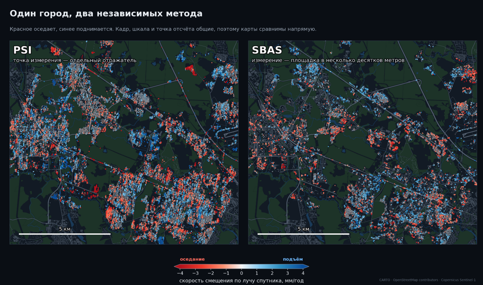
Let us look at the two radar imaging methods (fig. 1) used by L5: how they work, how they differ from each other, and above all, how we prove the calculations we obtain.
Two Methods: PSI and SBAS
Both methods work with the same images and answer the same question: how the distance from the satellite to the surface changed over the observation period. The difference lies in what each one treats as a reliable measurement point.
PSI looks for stable reflectors — places that return the radio signal in the same way from one acquisition to the next, for years. In a city these are building corners, roof parapets, balcony structures, supports, manholes, and fences. Each such reflector becomes a separate measurement point the size of an image pixel. In the 13 × 13 km Zelenograd frame there are 188 thousand such points, and they are distributed unevenly: over built-up areas the density is several times higher than the frame average.
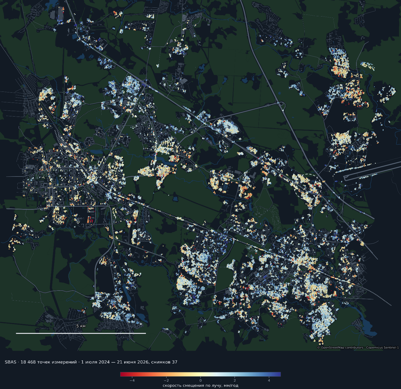
SBAS works not with individual points but with patches: images are combined in pairs, and the phase is averaged over a cell of several tens of meters. A reflector does not have to be perfect — what matters is that the patch as a whole behaves predictably. That is why SBAS sees where PSI is silent: fields, spoil heaps, roads, and slopes without buildings.
We run the analysis using both methods and compare the results with each other. This is not duplication: where two independent calculations agree, the result can be trusted without reservations.
Check One: Satellite vs. Ground Station
The surest way to verify satellite measurements is to compare them with ground measurements obtained in a completely different way. In Zelenograd and its surroundings, global navigation satellite system stations are in operation: they continuously record their position with daily resolution.
We took a station that does not participate in the calculation at all and compared its movement with what the satellite showed within a 250-meter radius around it. To make the comparison valid, both quantities are taken in the same way: the movement of this station relative to a reference point ten kilometers away. This is needed to keep the check fair: both systems answer the same question — how much one place has gone down relative to another.
The result is based on four calculations: the PSI method diverged from the station by 0.50 mm/year on the descending orbit and by 0.28 mm/year on the ascending one, and the SBAS method by 0.31 and 0.03 mm/year. The inherent error of the ground measurements over this interval is ±1.1 mm/year. That is, the difference between two independent measurement systems is three times smaller than the error of the one we are comparing against. Two orbits are two independent checks of the same object. The satellite passes over the city on ascending and descending trajectories, looking from different sides and at different times of day. If a building moves vertically, both acquisitions will show it identically; if the movement is horizontal, the signs will diverge. This is how we separate subsidence from sideways displacement.
This is the answer to the question “can this be trusted”: the approach confirms its reliability — the results are verified not in theory but on a real site, through independent calculations, which is visible at the level of an individual building.
What Is Visible at the Level of an Individual Building
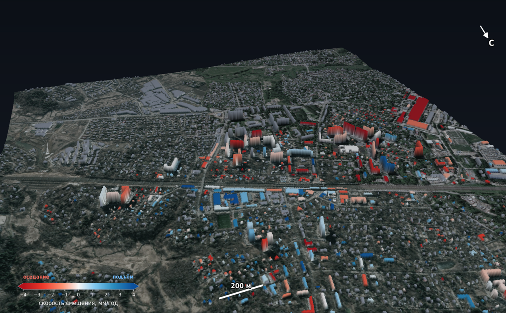
Cities do not subside as a whole: neighboring buildings can behave differently depending on age, construction, and the ground under the foundation. We reduce measurement points to objects: each building gets its own velocity — the median over the points on it and within a 30-meter strip around it.
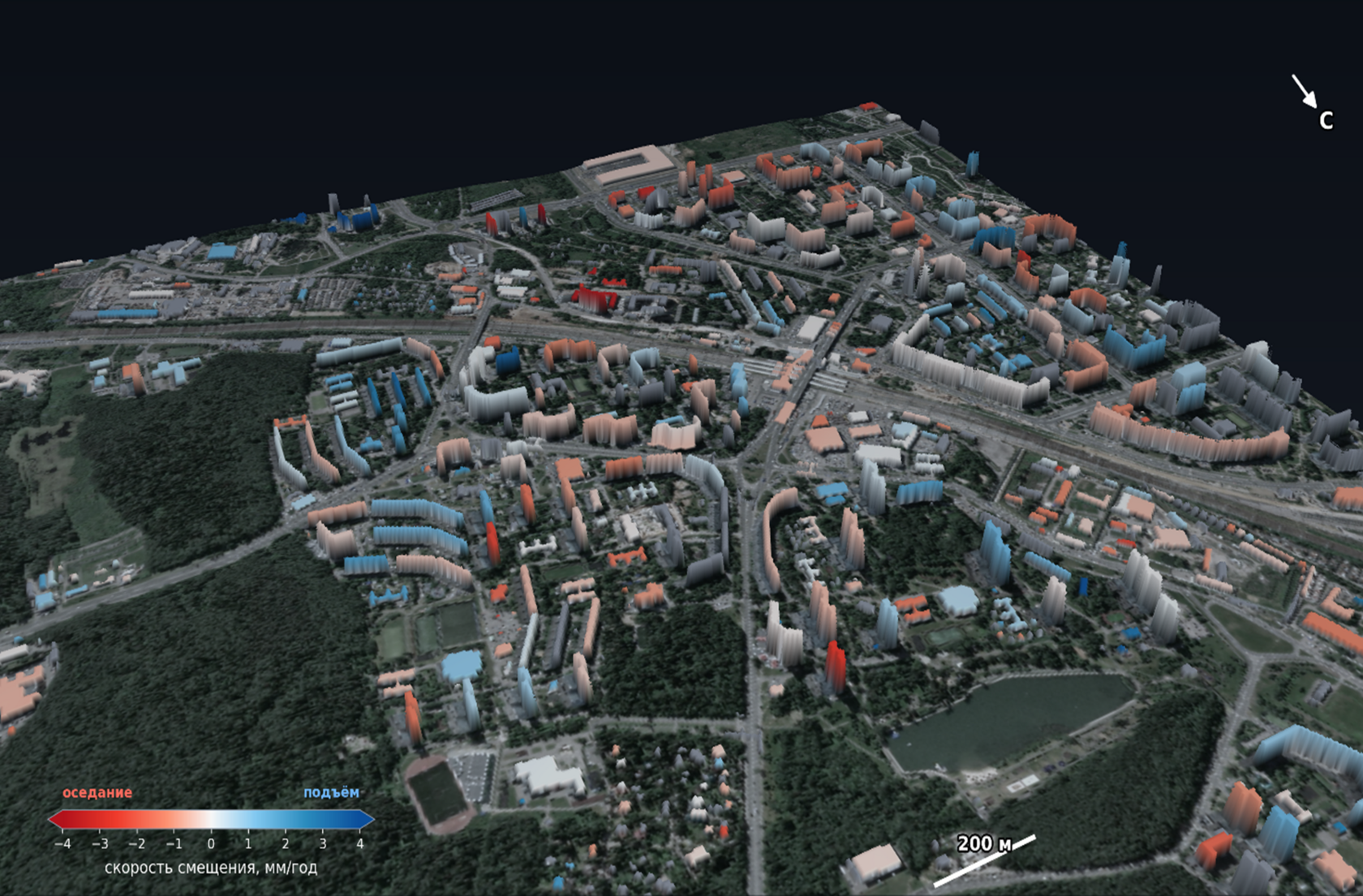
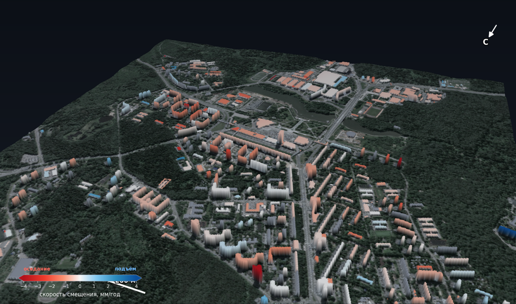
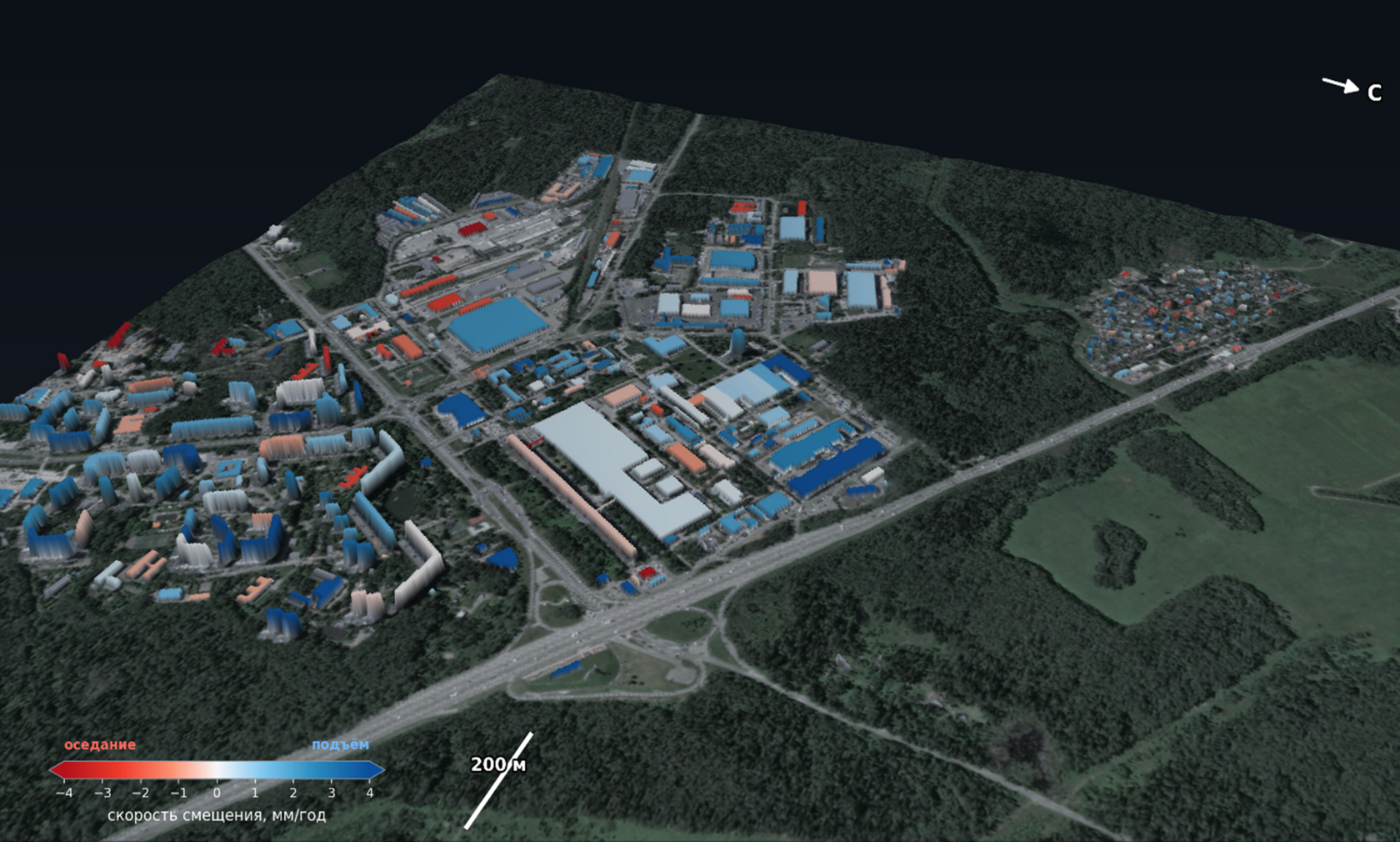
In Zelenograd, 81% of measured buildings have a velocity of less than 2 mm/year in absolute value. Movement distinguishable from noise on both orbits and in the same direction is present in 462 buildings. For each of them we provide the address, coordinates, velocity with its error, and a time series by date.
Why Buildings “Rise”
The first question that may arise on closer study of our images: how can a building rise? The answer has three components, which also explain the principle of the two-orbit calculation.
Part one: the reference is always relative. The satellite does not measure absolute height — it measures the change in distance to the surface. The area where the change in the surface is minimal or zero is set by us on the map. Zelenograd subsides fairly weakly: the median across buildings is minus half a millimeter per year. So a building that is simply standing ends up “above zero” and is colored blue.
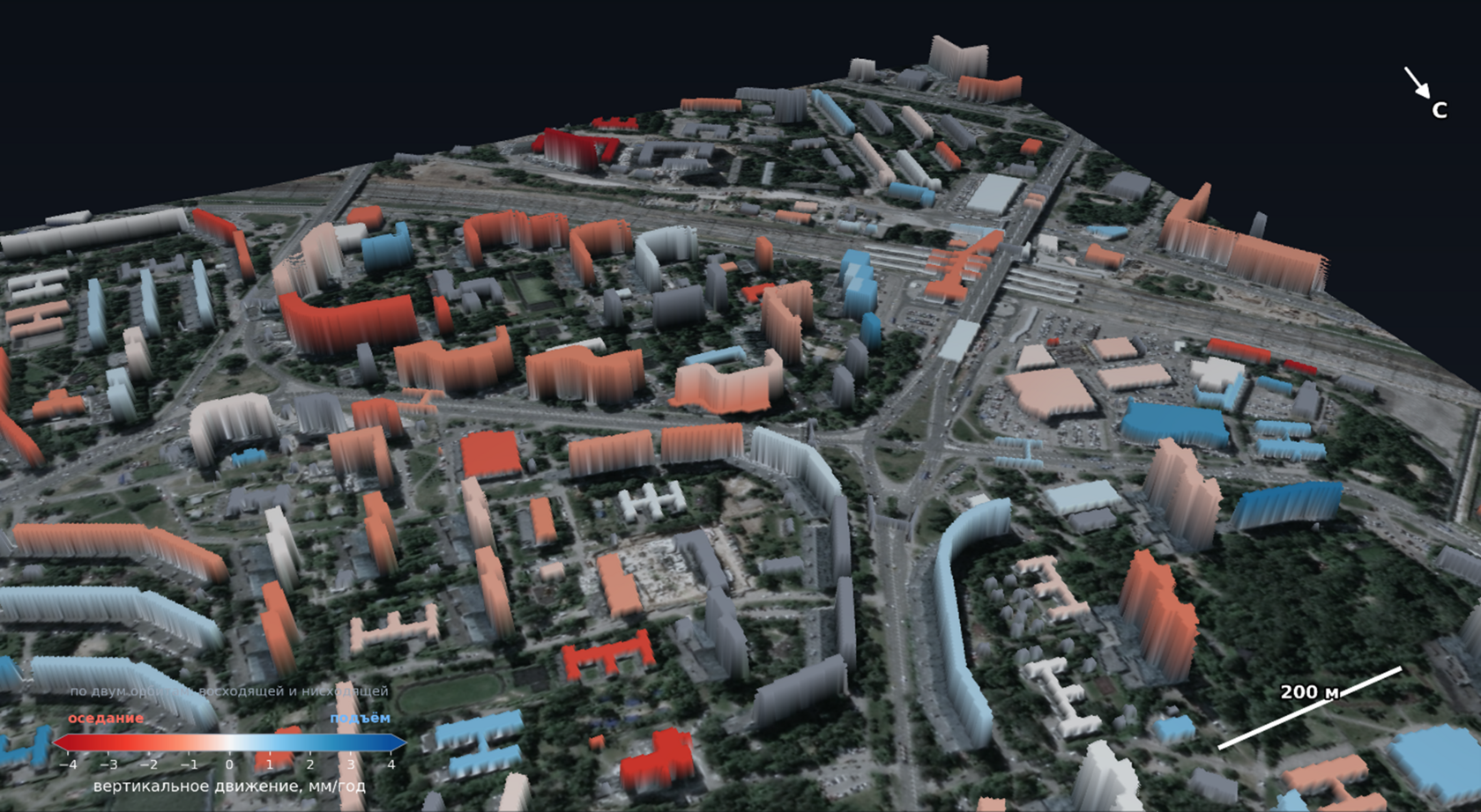
Part two: the beam is not vertical. The satellite looks at the ground at an angle of about 35–45 degrees and measures movement along its own beam. This quantity includes both vertical and horizontal movement. One orbit cannot separate them: a building sliding sideways and a building going up will give a similar result.
Part three: two orbits solve the problem. The descending orbit looks at the city from the east, the ascending from the west. Two measurements of the same building from different sides give a system of two equations, from which the vertical and horizontal components are found separately. Fig. 7 shows the result of such a decomposition: the color of a building is no longer movement along the beam, but the true vertical.

The rise here is neither an accident nor an error. While construction is under way, water is pumped out of the excavation, and the ground around it subsides. After the development is completed, pumping stops, the groundwater level recovers, and the base swells — the building rises with it by several millimeters a year. The effect fades over several years, and it is useful to observe: it shows that settlement is complete and the base has reached equilibrium.
There is also a third, seasonal cause of rise. For light structures on shallow foundations — hotels, warehouses, hangars — frozen ground heaves in winter and lifts the building by a couple of millimeters, and in summer everything returns. We can observe this by acquisition dates: in winter such structures rise 2 mm above their own baseline, in summer they drop 3 mm below it. High-rises on piles driven below the freezing depth show no seasonal movement at all.
The practical conclusion is simple: one orbit answers the question “is it moving”; two orbits answer the question “where exactly”. That is why we carry out displacement studies using two orbits.
Work at an Industrial Site: the Open-Pit Mine
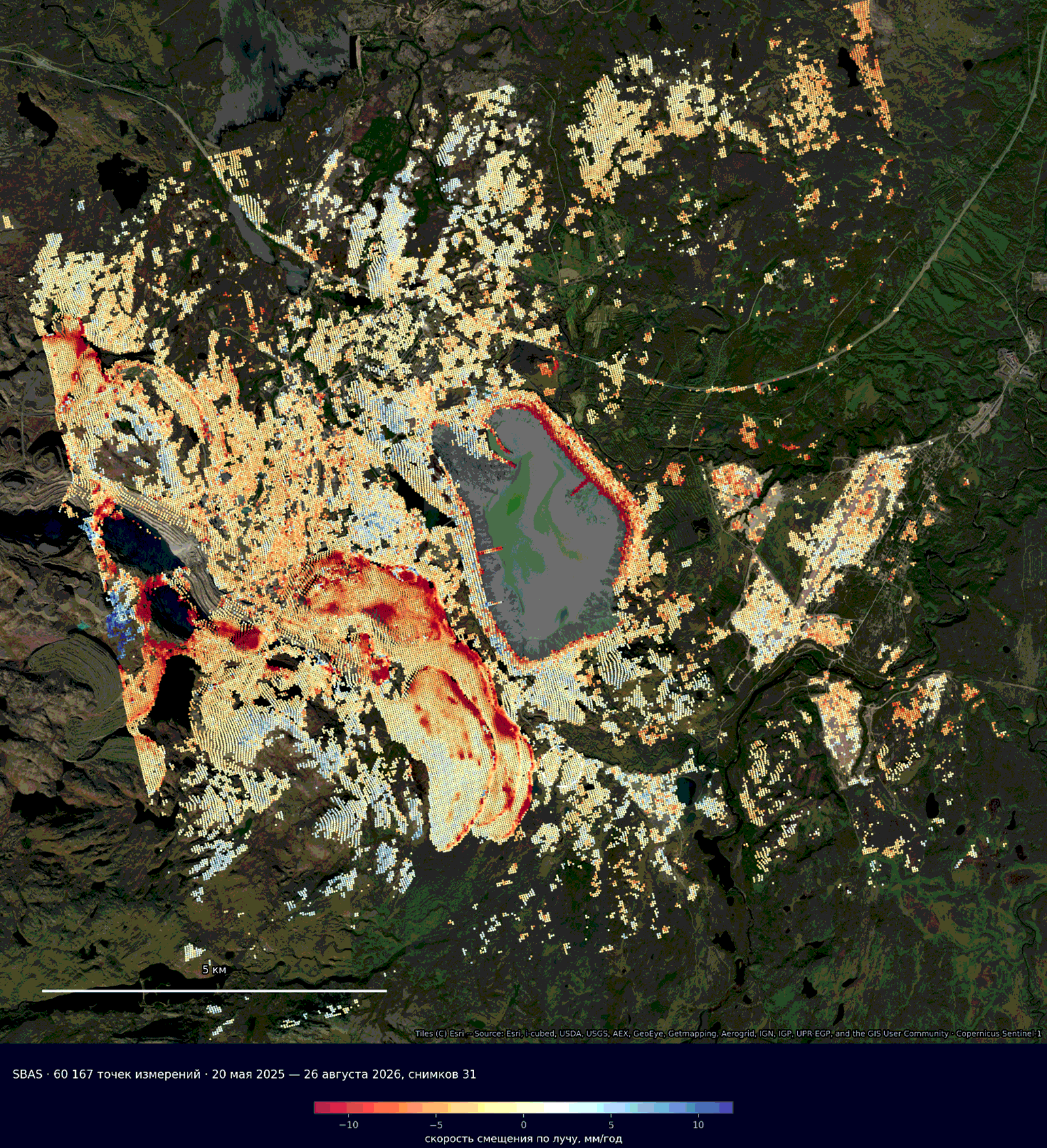
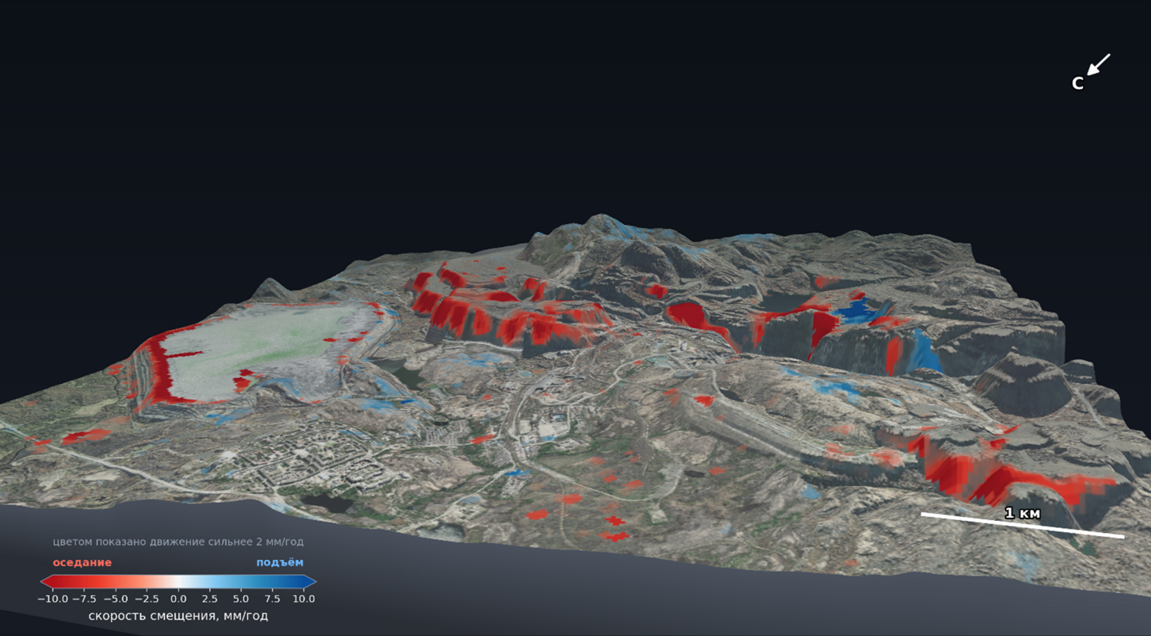
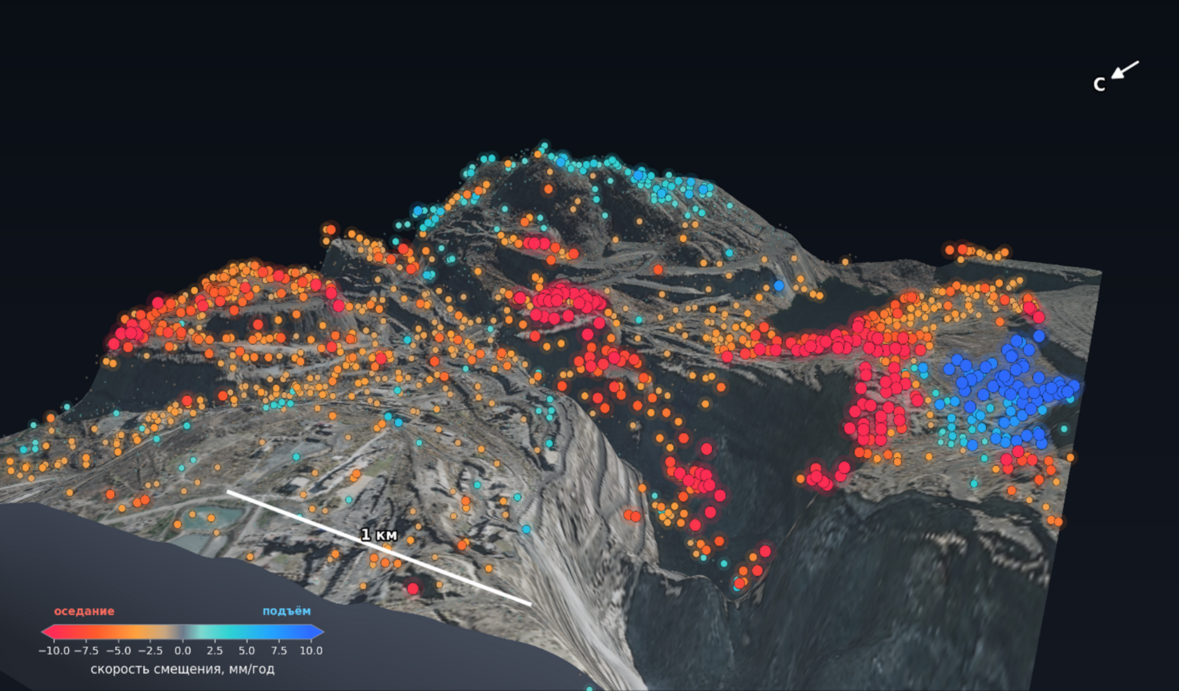
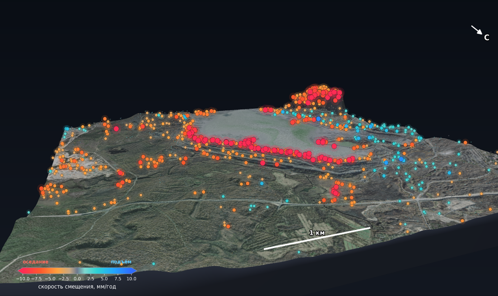
A city is a test. Where movement is fast and costly — open pits, spoil heaps, tailings storage facilities, slopes — the same millimeters turn into an early warning. We processed the open-pit mine in Zapolyarny: a site with an elevation difference of 380 meters and 60 thousand measurements by the SBAS method.
What the Customer Receives
- A velocity map for the entire site: PSI, SBAS, or both methods, georeferenced for loading into a GIS.
- A movement series for each point and each object: not only “how many mm per year”, but also how it accumulated by acquisition date.
- Objects, not pixels: a register of buildings or zones with addresses, areas, velocities, and errors, ready for a table and a report.
- Direction of movement, not only magnitude — where two orbits are available: vertical and horizontal separately.
- Automatic identification of movement zones with an assessment of whether the process is accelerating or not, and with an honest indication of where the data is insufficient.
- History backward: time series can be calculated without a single site visit.
- Recalculation as new images arrive.
Timeline: the first result for a new site — from a few days.
Limitations of the Method
- A reflective surface is required. Forest, water, freshly plowed fields, and smooth sand do not hold the signal. In a city this is not a problem; on open ground it is a limitation that SBAS addresses.
- Winter in the north gets in the way. Snow and ground freezing produce a false trend; these dates are excluded, and in winter the temporal resolution drops.
- The method sees the surface, not the structure inside. It will show that a building or a pit wall is moving, but the cause is determined by a specialist on site.
- Fast displacements (tens of centimeters between acquisitions) require a separate methodology, which is currently under active development at our company and will be available in the near future.